Linear Models

Author

Mathieu Ribatet

🏘️ Apartment prices in Warsaw

In this Lab we are going to play with a data set which contains the prices of the apartments which were sold in Warsaw, Poland, during the calendar years 2007 to 2009. Overall we have 409 observations on the following 6 variables :

surface area of the apartment in square meters.
district a factor corresponding to the district of Warsaw with levels Mokotow, Srodmiescie, Wola and Zoliborz
n.rooms number of rooms in the apartment
floor floor on which the apartment is located
construction.date year that the apartment was constructed
areaPerMzloty area in square meters per million zloty

The dataset can be retrieved from the following piece of code:

rm(list=ls())##clear memory before working
url <- "https://mribatet.perso.math.cnrs.fr/CentraleNantes/Data/Warsaw.csv"
data <- read.csv(url, row.names = 1)

Hint: It may be tedious to write code like data$areaPerMzloty so we might want to “attach” the data set to your R session so that we can just use variable names, e.g., areaPerMzoloty . This is done using the following code

attach(data)

Of course you can “detach” the data set by invoking

detach(data)

Familiarized yourself with the dataset. What are the type of the variables? Which ones are the explanatory variables, i.e., $x_j$ in the lecture ? Which one is the response variable, i.e., $Y$ in the lecture ?
Plot the evolution of the price w.r.t. the district and comment.
```
##Write code here
```
Plot the evolution of the price w.r.t. construction date and comment.
```
##Write code here
```
Plot the evolution of the price w.r.t. the number of rooms and comment.
```
##Write code here
```
Plot the evolution of the price w.r.t. the surface and comment.
```
##Write code here
```
Read the documentation of the lm function and fit your first linear model where you model the price as a function of all the covariates (you will store it in a object called fit)
```
##Write code here
```
Run the following code and say what it does. Compute by yourself the hat matrix and compute its trace. Was it expected? Compute the sum of each row? Again was it expected?
```
X <- model.matrix(fit)

##Write code here
```
Run the following code and comment. Make sure you understand every single output.
```
summary(fit)
```
What are the meaning of the “*”? Is the surface statistically significant? Why do we have 401 degrees of freedom for the residual standard error? Look at the bottom line where one can read p-value: < 2.2e-16, what does it say?
Why are we having lines named districtSrodmiescie, districtWolaand districtZoliborz? Why there is no districtMokotow? Is the variable district statistically significant?
What can you say about your fitted model? Produce diagnostic plots using the following code
```
plot(fit)
```
We see that our model is not very accurate. We may need to work with a more complex model by considering “new variables” such as log(surface). Nowadays, this stage is known as feature engineering–a few years ago we didn’t use a name for such a basic stage ;-)

Using the update function, try to get a better fitted model by incorporating new variables; you will call this new model new_fit.

For instance, you may want to consider the log, square or even product between two variables such as the surface * n.rooms (in statistics it is called an interaction). You may also want to “merge” some levels of a categorical variable, e.g., merging levels Wola, Zoliborz and Mokotow into a single level.
```
## Write code here
```
Perform model selection between models fit and new_fit using an information criterion and, if relevant, analysis of variance.
```
##Write code here
```
Read the documentation of the step function and next perform stepwise model selection. From this output plot the price of the apartments to predictions. Interpret the effect of the floor variable on the price.
```
##Write code here
```
Perform residual analysis for your best model. Comment and do a scatterplot of prices w.r.t. predictions (the function predict may be useful for this purpose).
```
## Write code here
```

🎁 Bonus: Additive models

It is a bit unfortunate that your best linear model is not extremely powerful. The linear model is widely used and highly interpretable but often lacks some flexibility. More flexible models exist but the price to pay is a decrease in interpretability. Neural networks are the typical example of powerful models but not interpretable at all. A good compromise are additive models:

\[ Y = f_1(X_1) + \ldots + f_p(X_p) + \varepsilon, \qquad \varepsilon \sim N(0, \sigma^2), \]

where $f_j$ are unknown functions to be estimated. We will not cover the theory beyond this model but I just want you to know that those functions are defined in a given basis and, as so, parameters of the above models are the coefficient in that basis for each function $f_j$ (and consequently we get a linear smoother).

Fitting such model is a piece of cake using the mgcv library (that comes with R but is not loaded in memory):

library(mgcv)

Loading required package: nlme

This is mgcv 1.9-1. For overview type 'help("mgcv-package")'.

add_mod <- gam(areaPerMzloty ~ s(surface) + s(construction.date) + district + s(floor), data = data)
summary(add_mod)


Family: gaussian 
Link function: identity 

Formula:
areaPerMzloty ~ s(surface) + s(construction.date) + district + 
    s(floor)

Parametric coefficients:
                    Estimate Std. Error t value Pr(>|t|)    
(Intercept)         113.0161     1.2653  89.319  < 2e-16 ***
districtSrodmiescie -10.9918     2.1346  -5.149 4.17e-07 ***
districtWola          2.8025     2.5346   1.106    0.270    
districtZoliborz     -0.5875     3.1731  -0.185    0.853    
---
Signif. codes:  0 '***' 0.001 '**' 0.01 '*' 0.05 '.' 0.1 ' ' 1

Approximate significance of smooth terms:
                       edf Ref.df      F  p-value    
s(surface)           7.043  8.081  3.937 0.000143 ***
s(construction.date) 8.472  8.922 19.186  < 2e-16 ***
s(floor)             2.011  2.518  1.578 0.232662    
---
Signif. codes:  0 '***' 0.001 '**' 0.01 '*' 0.05 '.' 0.1 ' ' 1

R-sq.(adj) =  0.443   Deviance explained = 47.1%
GCV = 287.87  Scale est. = 272.72    n = 409

Without knowing the theory (which is unfortunate of course), we can guess what’s going on with the above output. For instance one can see that the (adjusted) $R^2$ is around 45% and that the floor variable, even within a additive form, is not statistically significant. The variables surface and construction.date are strongly significant. So we can update our model by removing the s(floor) term and next have a look the effect of the two aforementioned variables.

add_mod <- update(add_mod, . ~ . - s(floor))
par(mfrow = c(1, 2), mar = c(4, 5, 0.5, 0.5))
plot(add_mod)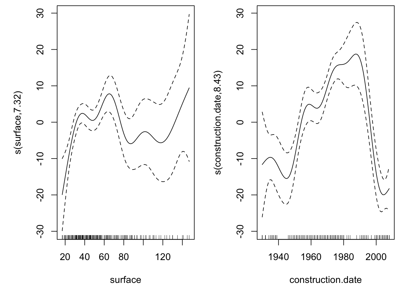

From the above (right) graph we can see that the cheapest apartments are those built around 1980 while much older or recent ones are more expensive.