MathALEA – Introduction to R

Author

Mathieu Ribatet

Introduction

R is a powerful and widely used programming language and software environment for statistical computing and data analysis. Developed by statisticians, R provides a vast array of tools for data manipulation, visualization, and modeling. Its open-source nature and extensive package ecosystem make it a popular choice among researchers, data scientists, and analysts. With its strong community support and integration capabilities, R is ideal for handling complex datasets, performing advanced statistical tests, and creating high-quality visualizations.

Installation and User Interface

Although extremely powerful, R has a terrible user interface and it is (highly) recommended to use a different GUI. Several options exist and, as I am writting this document, RStudio from Posit is one of the most popular (not my taste though). We will use it in this course.

Therefore the installation is a two steps procedure:

Watch this video to get a quick glimpse at the functionalities offered by the RStudio GUI.

The R language (well actually S ;-)

Disclaimer: You won’t learn how to do scientific programming with R in this course. Yet you will have to get a minimal knowledge. This is the aim of this section!

## Of course you could use R as a calculator but this is *NOT* scientific programming
1 + exp(2 * sin(3.5 * pi^2))

[1] 2.028197

## Create variables using either '<-' or '=' ('<-' is the historical assigment operator)
a_string <- "zoo"
a_number <- 4.5
a_vector <- c(1, 3, 5)##'c' might stand for concatenate
a_repetitive_vector <- rep("a", 5)
a_sequence <- 3:5##integer between 3 and 5 *inclusive* (not like Python)
a_matrix <- matrix(a_sequence, 2, 3)##a 2 x 3 matrix (note how recycling was used and how the matrix is populated by columns unless specified)

We see how to create character strings, vector, matrices… but other objects exist as well: namely data frame and lists. Data frames appear to be like a matrix but are more flexible than matrices since columns may be of different types, i.e., the 1st column contains real numbers while the 2nd character strings. This is not possible with matrices which makes data frames very appealing since data are likely to be of different kind.

## Create a data frame
df <- data.frame(1:5, letters[1:5])
df

  X1.5 letters.1.5.
1    1            a
2    2            b
3    3            c
4    4            d
5    5            e

## Trying to force a matrix to be a data frame, look at what happens
a_matrix

     [,1] [,2] [,3]
[1,]    3    5    4
[2,]    4    3    5

a_matrix[1,1] <- "a"##setting the (1,1) element to be a character
a_matrix## oupppsss every entries have been converted to character strings !

     [,1] [,2] [,3]
[1,] "a"  "5"  "4" 
[2,] "4"  "3"  "5"

Lists are the most flexible objects (and again that come with a CPU cost). Roughly speeking, you can do whatever you want with list and it is like a data frame but now columns may have different sizes.

a_list <- list(a_matrix, a_string, df)

No that you know how to create object you may want to manipulate it.

## Access element of a vector/matrix
a_vector[2]##the 2nd element, index starts à 1 not 0 like Python

[1] 3

a_matrix[2,1]##2nd row, 1st colum

[1] "4"

a_matrix[,1]##the 1st column

[1] "a" "4"

a_matrix[,-c(1, 3)]##the matrix without the 1st and 3rd columns

[1] "5" "3"

## For lists we have to use double brackets
a_list[[3]]##the 3rd component of the list, i.e, df

  X1.5 letters.1.5.
1    1            a
2    2            b
3    3            c
4    4            d
5    5            e

a_list[[3]][1, 2]## the 1st row and 2nd column of df

[1] "a"

When doing scientific programming, having expression like a_list[1,2] is barely understandable. Similarly to the name you give to your objects/variables (or your child, bad joke I know), it is good practice to give sensible names to the columns / rows / components of a data frame / list.

## Creating a list with component names 
named_list <- list(name1 = 1:4, name2 = rep("toto", 3))

## Setting names to an 'unamed' list
names(a_list) <- c("toto", "tata", "tutu")

## We can now access the component by its name
a_list$toto## exactly the same as a_list[[1]]

     [,1] [,2] [,3]
[1,] "a"  "5"  "4" 
[2,] "4"  "3"  "5"

## For data frame we can use as before or using colnames (colnames works with matrix as well)
colnames(df) <- c("var1", "var2")

## We can do the same with rows
rownames(df) <- paste("row", 1:5)

## Now we can access columns in two ways
df$var1##as for list

[1] 1 2 3 4 5

df[,"var1"]##new way, works for matrices as well

[1] 1 2 3 4 5

df["row 1",]##1st row selected from its name

      var1 var2
row 1    1    a

We are all set to do some algebra!

A <- matrix(runif(16), 4)##4x4 matrix populated with random numbers
x <- 1: 4##vector of size 4

1 + A##elementwise addition (add 1 to all entries)

         [,1]     [,2]     [,3]     [,4]
[1,] 1.494632 1.398461 1.933961 1.316626
[2,] 1.955489 1.200661 1.159848 1.622020
[3,] 1.169939 1.946064 1.115951 1.839180
[4,] 1.350695 1.817112 1.702661 1.136545

diag(A)##diagonal of A

[1] 0.4946317 0.2006611 0.1159515 0.1365450

t(A)##transpose of A

          [,1]      [,2]      [,3]      [,4]
[1,] 0.4946317 0.9554893 0.1699386 0.3506947
[2,] 0.3984613 0.2006611 0.9460643 0.8171120
[3,] 0.9339608 0.1598479 0.1159515 0.7026607
[4,] 0.3166260 0.6220198 0.8391804 0.1365450

B <- t(A) %*% A##matrix multiplication
solve(B)##inverse of B

          [,1]      [,2]      [,3]      [,4]
[1,]  4.017197  2.574321 -2.728396 -4.259161
[2,]  2.574321  4.091991 -2.895960 -4.505569
[3,] -2.728396 -2.895960  3.285986  3.292698
[4,] -4.259161 -4.505569  3.292698  6.845208

svd(A)##singular value decomposition

$d
[1] 2.0514516 0.8601088 0.8198060 0.2568064

$u
           [,1]       [,2]       [,3]       [,4]
[1,] -0.5126352  0.5528186  0.1596958 -0.6372550
[2,] -0.4514127 -0.3627312  0.7780650  0.2434492
[3,] -0.5265872 -0.6254247 -0.5191582 -0.2490473
[4,] -0.5061004  0.4143207 -0.3155739  0.6874692

$v
           [,1]        [,2]        [,3]       [,4]
[1,] -0.4639933 -0.03967854  0.76058039  0.4523862
[2,] -0.5881554 -0.12283891 -0.64558720  0.4713820
[3,] -0.4716728  0.78703657 -0.01026684 -0.3974830
[4,] -0.4650894 -0.60324924  0.06803843 -0.6443237

chol(B)##Cholesky decomp

         [,1]      [,2]      [,3]       [,4]
[1,] 1.144328 0.7306916 0.7697301  0.8227024
[2,] 0.000000 1.1080775 0.4743686  0.5011633
[3,] 0.000000 0.0000000 0.7664861 -0.3686970
[4,] 0.000000 0.0000000 0.0000000  0.3822141

eigen(B)##eigen decomposition

eigen() decomposition
$values
[1] 4.20845364 0.73978709 0.67208180 0.06594953

$vectors
           [,1]        [,2]        [,3]       [,4]
[1,] -0.4639933  0.03967854  0.76058039  0.4523862
[2,] -0.5881554  0.12283891 -0.64558720  0.4713820
[3,] -0.4716728 -0.78703657 -0.01026684 -0.3974830
[4,] -0.4650894  0.60324924  0.06803843 -0.6443237

R, as any high level language, has “vectorial” capabilities, i.e., can apply operations on vectors without using a loop. This is a bless and a curse. A curse because you write “math” that will give you a 0 on a exam (think about writing \(1 / A\) when \(A\) is a matrix :-( ). But a bless as you can code quite complex stuffs without any for/while loop (and get a fast code).

To sum up, R is high-level so you have to use its vectorial abilities otherwise just stick with low level languages as C.

a_grid <- seq(0, 2 * pi, length = 500)
cos(a_grid)##evaluate cosinus on a grid

Alright we are ready to go a bit further to do scientific programming: writing our own functions, use for/while loops, if else statements and so on…

my_f <- function(arg1, arg2_with_default = 1){
  ## This function return the maximum (without using the builtin max function...)
  ## function can output only one object so if needed output a list
  
  if (arg1 > arg2_with_default){
    ans <- arg2_with_default
  } else##if only one line, curly brackets can be omitted
    ans <- arg2_with_default
  
  return(ans)
}

## A call
my_f(2, 3)##max(2, 3)

[1] 3

my_f(2)##max(2, 1)

[1] 1

my_f(arg2_with_default = 5, 1)##max(1, 5)

[1] 5

For and while loops look like…(by the way never use a while loop if you know how many iterations you’ll do!)

for (i in 1:100){
  print(i)
}

for (letter in LETTERS[1:5]){
  print(letter)
}

i <- 10
while (i > 0){
  print(i)
  i <- i - 1
}

Graphics

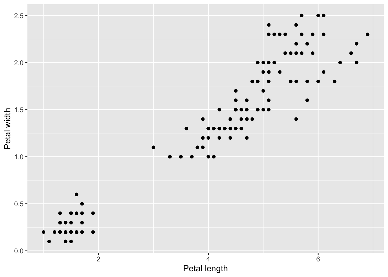
As expected, R can do beautiful graphics including statistical ones such as boxplot, histogram. I cannot cover everything of course but let me tell you one thing. There are built in graphics using base R and, now a trendy way of doing plots that is based on the “grammar of graphics” way. The latter relies on the third party library ggplot2 that you need to install and load. Personnaly I am not very fond of ggplot because it is too verbose for my personnal taste, but people seem to like it so I have to mention it.

## Scatter plot
plot(iris$Petal.Length, iris$Petal.Width, xlab = "Petal length", ylab = "Petal Width")

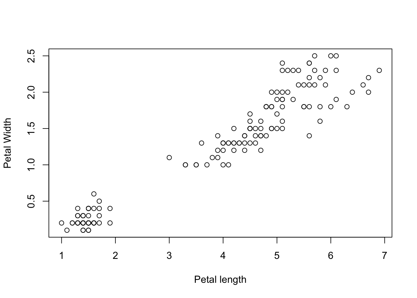
## ggplot way would be
library(ggplot2)
ggplot(iris) + geom_point(aes(Petal.Length, Petal.Width)) +
  labs(x = "Petal length", y = "Petal width")

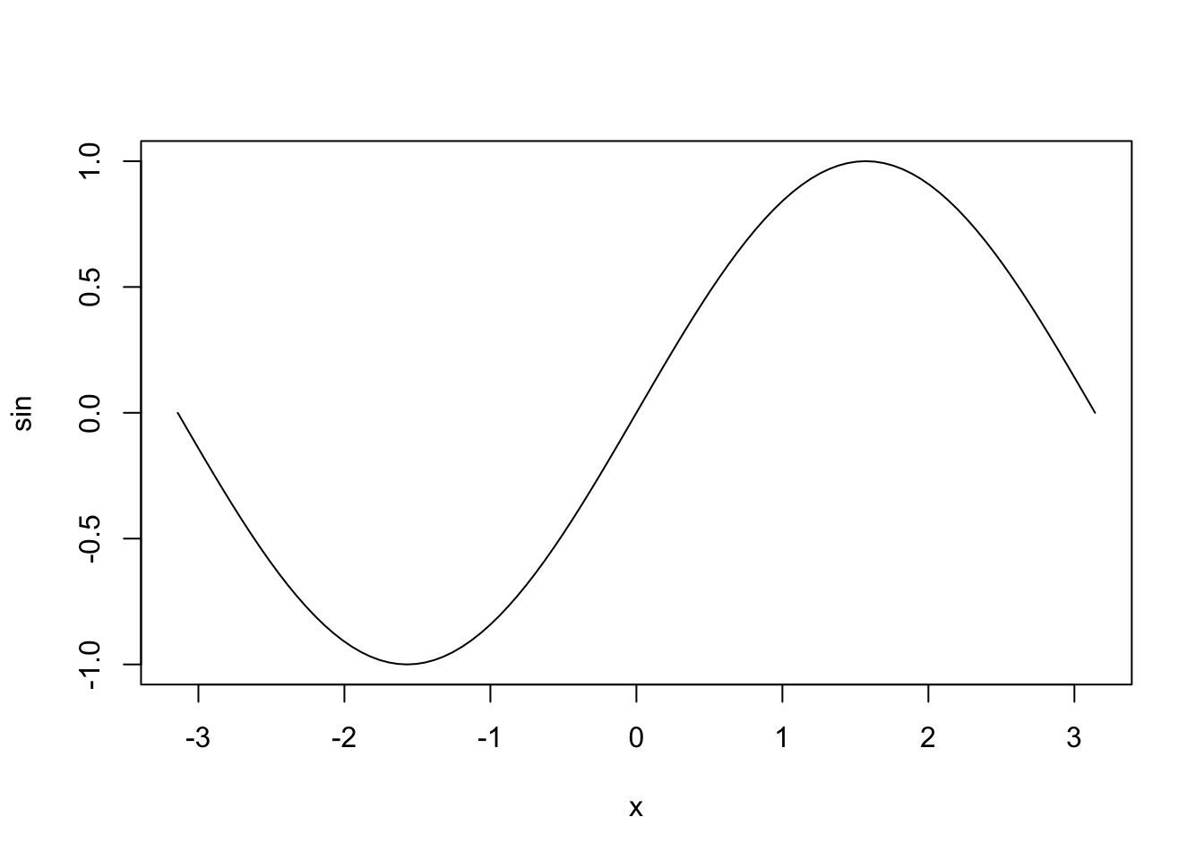
## We can plot a function without evaluating it
plot(sin, from = -pi, to = pi)##Python why you don't have that--grrrrr

Of course, I won’t cover every possible plots but here are some just to tease you

boxplot(Sepal.Width ~ Species, data = iris)

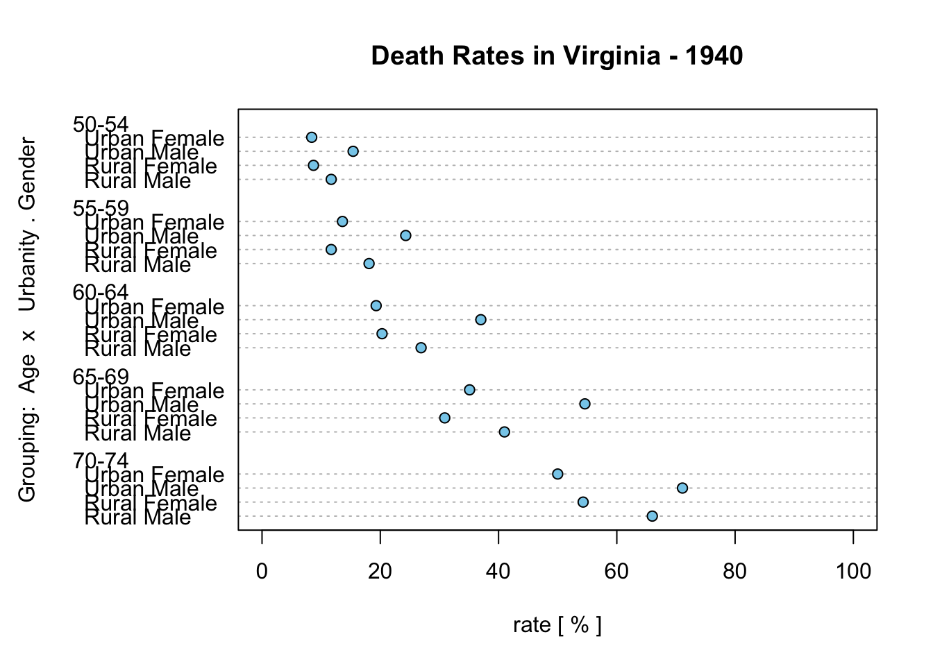
dotchart(t(VADeaths), xlim = c(0,100), bg = "skyblue",
         main = "Death Rates in Virginia - 1940", xlab = "rate [ % ]",
         ylab = "Grouping:  Age  x   Urbanity . Gender")

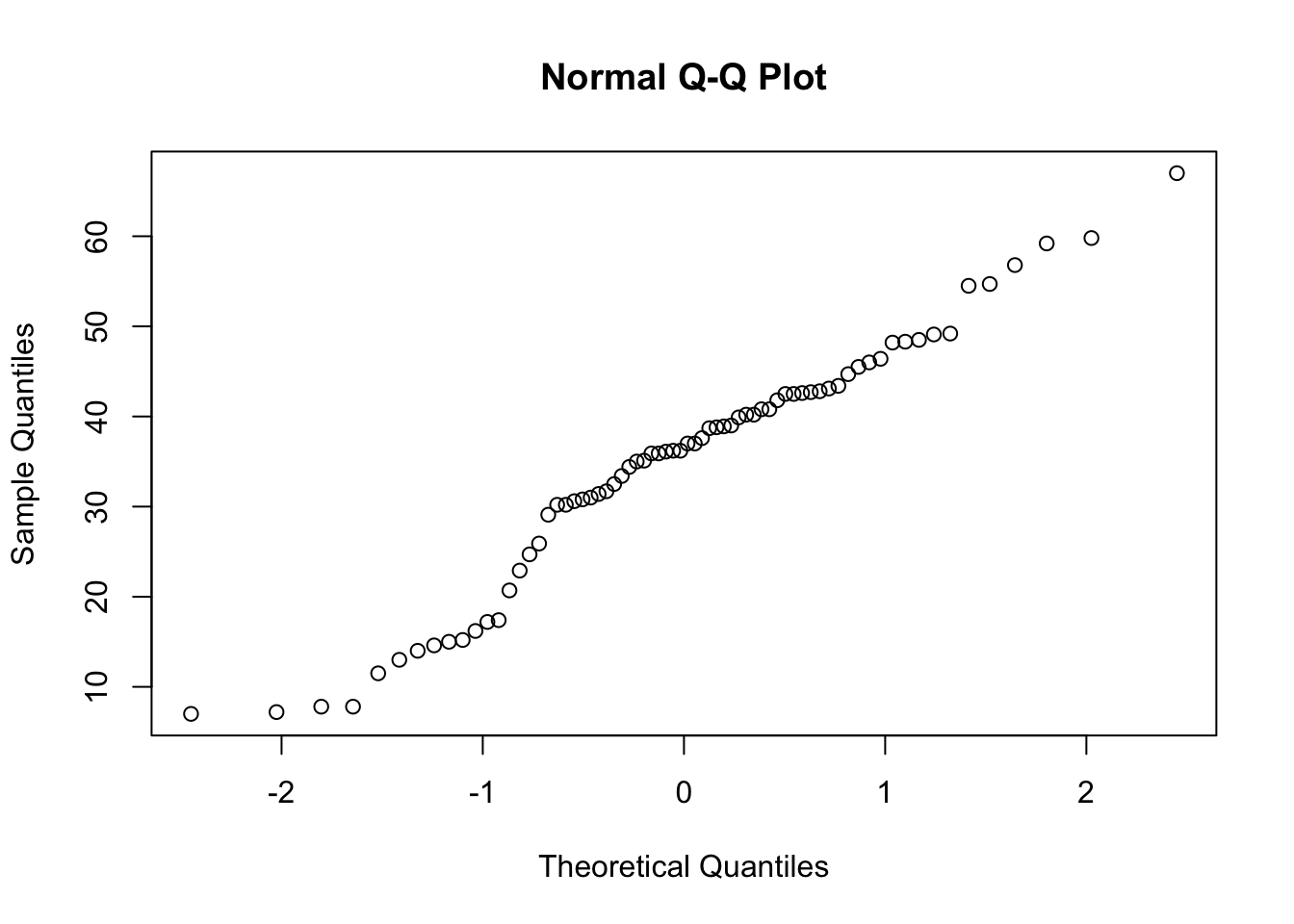
qqnorm(precip)

The most important…

…is what you are going to learn in statistics and how R will help you apply it! And if you want to dive a bit further you may want to have a look at this (tidyverse oriented though).